A Many-objective Optimization Approach for Single Source-trained Target EEG Classification

Authors: Monalisa Pal, Sanghamitra Bandyopadhyay and Saugat Bhattacharyya
Email: monalisap90@gmail.com, sanghami@isical.ac.in and saugatbhattacharyya@live.com

Welcome to this webpage which presents a many-objective optimization approach to perform Transfer Learning in Brain-Computer Interfacing domain. The objective of this work is to classify a subject's EEG using a classifier trained by an unrelated subject's EEG. The subject providing training-data for the classifier is called the source subject and the other subject whose intentions are classified is called the target subject. The major characteristics of this approach are as follows: it does not require multiple source subjects, it is not dependent on any specific feature and/or classifier, and it requires very less number of instances from the target subject during the training phase of supervised learning. This webpage contains a detailed description of the proposed approach along with its classification performance in a downloadable PDF file, the MATLAB code used for this work as a downloadable ZIP folder, and the step-wise illustration of the execution of the code.

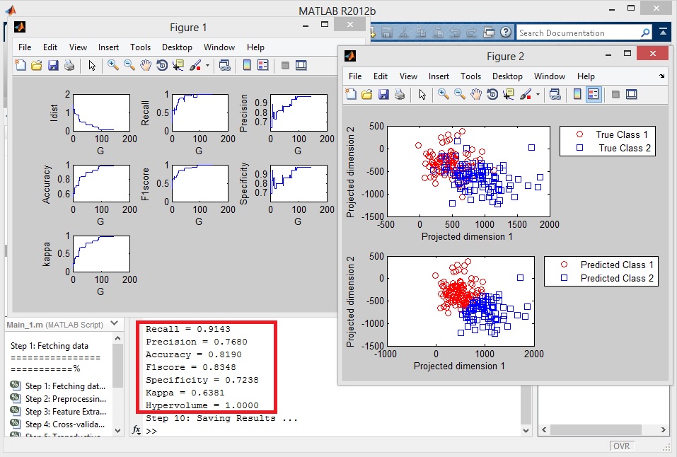
Description and performance of the proposed approach

A detailed description of the proposed approach is available as the supplementary material in the file named "Supplementary.pdf". Alongwith the description of the many-objective optimization approach, the supplementary material provides the classification results (Recall, Precision, Accuracy, F1-score, Specificity, κ-coefficient), the training and testing time requirements, and the quality of the solution obtained from the many-objective optimization approach (Hypervolume Indicator), for the overall understanding of this work.

Click here to download the supplementary material.

Specifications of the code

The experiment was conducted in a system having Intel Core i3 processor @ 2.3GHz with 4GB RAM and using MATLAB R2012b.

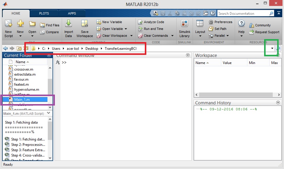
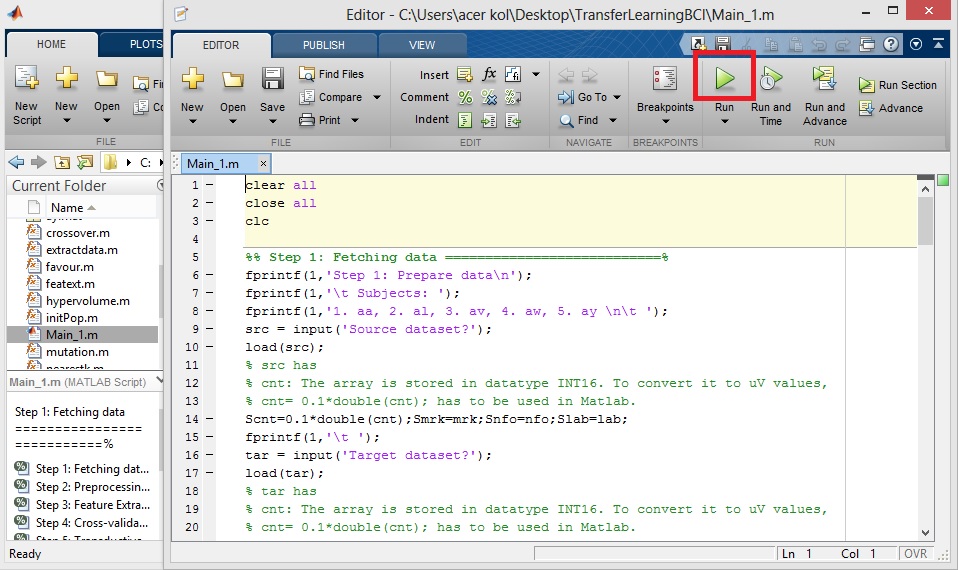
The MATLAB codes are available in a compressed folder named "TransferLearningBCI.zip" which is downloadable from the link below. The compressed folder is to be extracted in which there are 21 files (5 .mat files and 16 .m files). Here, the five .mat files correspond to the EEG recordings from five subjects from BCI Competition III (Dataset IVa). Description of the dataset is available on this link (as accessed on 7th December, 2016). From the remaining 16 .m files, the file named "Main_1.m" is the one to be executed and all the remaining ones are function definitions required for the entire execution. This program uses Welch's Power Spectral Density for feature extraction (defined in "featext.m" file) and linear support vector machine for classification (defined in "predictor.m" and "recognize.m"). Hence, if any other features and/or classifier is to be used, these 3 files ("featext.m", "predictor.m" and "recognize.m") are to be modified as per requirement.

Click here to download the MATLAB codes.

Getting help: For all the .m files, a brief description of the code can be looked up using the "help" command of the MATLAB as shown in the illustration below. It is important to browse into the location (or folder) where all the associated files are kept, before executing the "help" statement. To execute the help statement, the corresponding filename is to be typed, preceeded by the word "help".

Steps to execute the associated program

The code can be executed as listed below. Against each step, a screenshot is provided for reference. The screenshots are taken during execution of the code in Windows 8.

Open MATLAB. (Here, MATLAB R2012b has been used.)
Use the drop-down arrow (highlighted by green box) to browse to the location (highlighted by red box) where the ZIP folder has been extracted. Ensure there are 21 files in the location from the "Current Folder" pane, including a file named "Main_1.m" (highlighted by purple box) which is the file to be executed.
One of the ways to execute the file (Main_1.m) is to open the file in an Editor window (by double-clicking "Main_1.m" under "Current Folder" pane) and use the "Run" button of the Editor window (highlighted by red box). Alternatively, one can type the filename i.e. Main_1 in the "Command Window" when the prompt (>>) appears in order to execute the program.
Enter the subject's name you wish to choose as the source and the target subjects in the command window (highlighted by red box). These are actually the name of the .mat files which are the datasets corresponding to each subject. Note that all the previously entered commands can be seen from the "Command History" pane (highlighted by purple box).
Enter in the "Command Window" the dimension (parameter d as described in the proposed approach) of the space where the features are to be projected (highlighted in red box). Note that the step-wise execution of the program can be followed from the various statements printed in the "Command Window".
After all the user-inputs are provided, the transfer learning starts to decide the optimal weight for projecting the features into a d-dimensional space in order to maximize the source-trained target EEG classification performance.
At the end of the program execution, two graphs appear in separate windows called "Figure 1" and "Figure 2". "Figure 1" shows the optimization of different parameters with the iterations of the optimization algorithm and can be turned off by setting the plotflag argument to 0 of the transTL_wrap() function. "Figure 2" compares the true class labels against the predicted class labels and appears only when d=2. Beside the plots, the results of classification appear in the "Command Window" (highlighted by red box).
Inside the "Current Folder" pane, a new .txt file appears after execution of the code whose filename is in the format source_target_d. It records the results in a tab-delimited fashion in a row for every execution where the fields are in the following order: source id, target id, recall, precision, accuracy, F1-score, specificity, κ-coefficient and hypervolume.