Welcome to this webpage which presents two single-objective optimization approaches viz. UDE or Uniform Differential Evolution and its adaptive version (AUDE). These proposed algorithms have been applied on 19 benchmark problems and the efficacy of the approaches have been analysed in comparison to other Differential Evolution (DE) variants. Performance comparison of AUDE has also been done with the recent DE variant and the winner algorithm (LSHADE‐cnEpSin) of CEC 2017 competition. The primary highlight of the proposed approaches is the use of uniform distribution based reproduction strategies which have been supported by theoretical foundations and experiemental validations. This webpage contains the Python 3.4 code of the proposed approaches as a downloadable ZIP folder, and the step-wise illustration of the execution of the code. This webpage also contains the author-implemented version of LSHADE‐cnEpSin (in Python 3.4) as a downloadable ZIP folder.
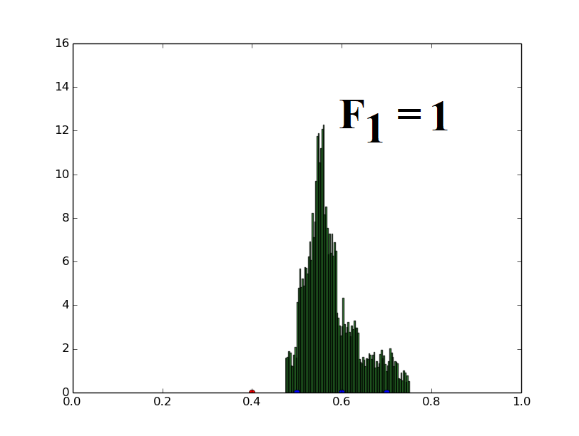
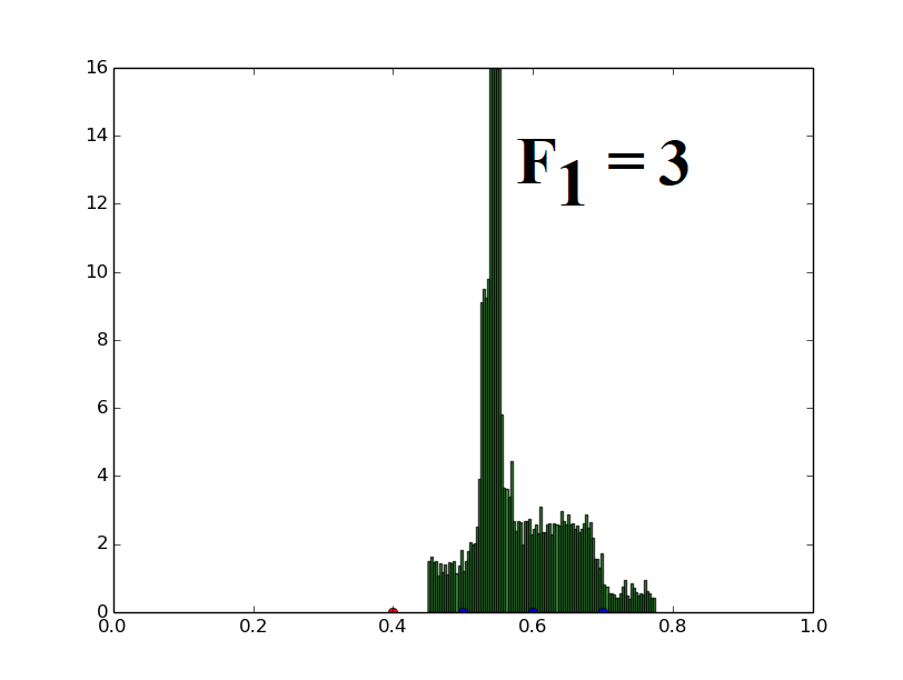
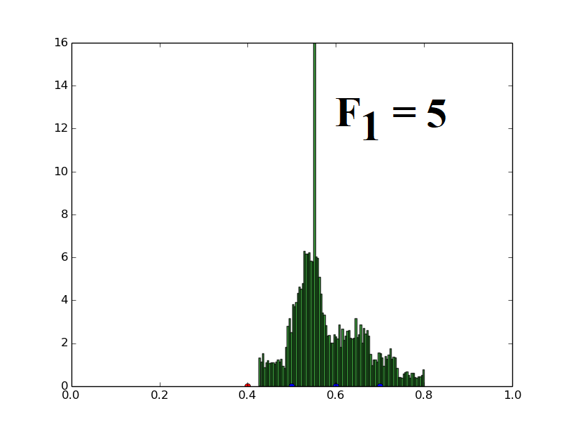
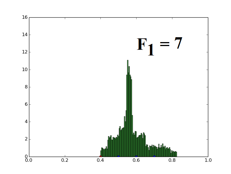
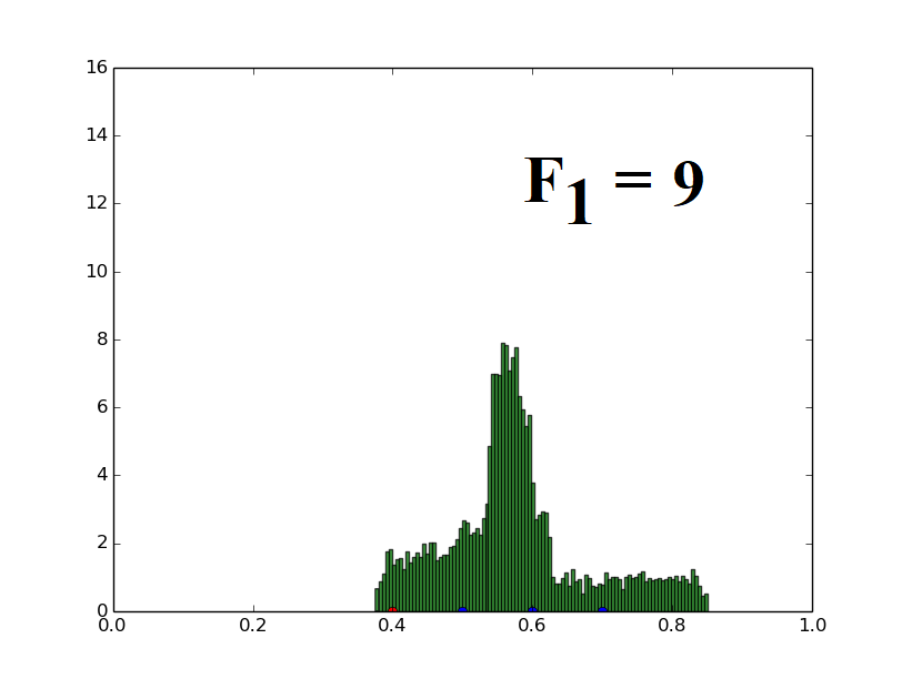
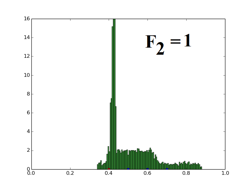
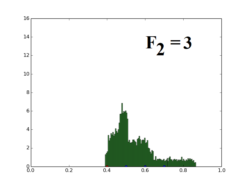
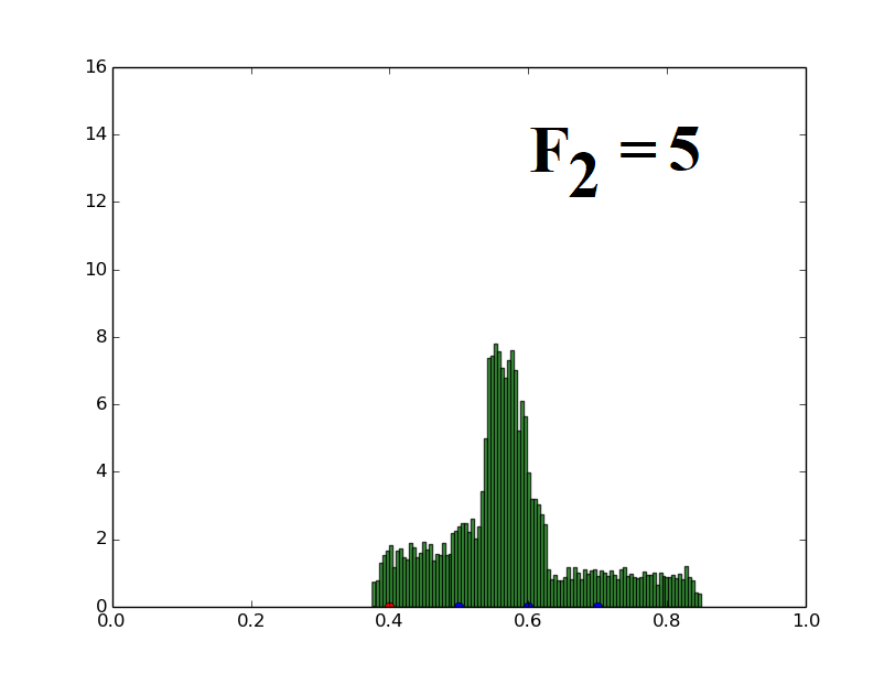
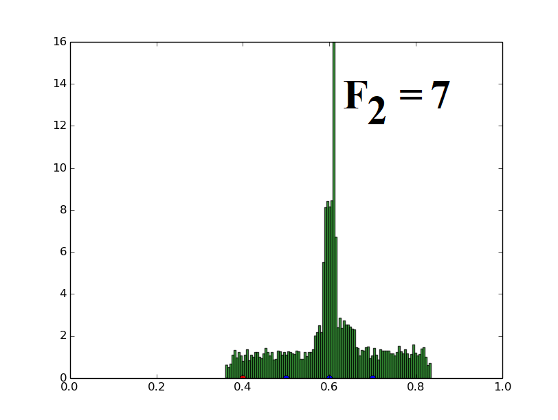
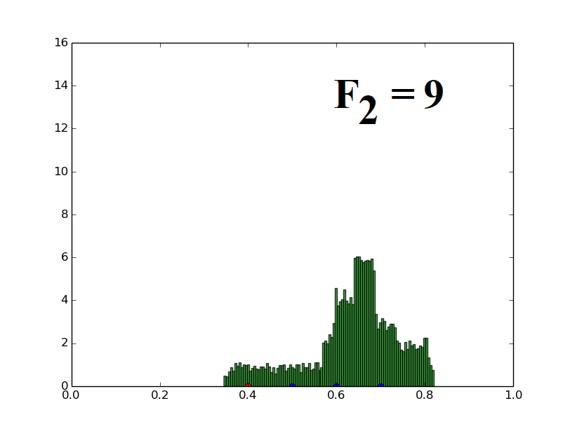
Population of one-dimensional decision variables is used to generate histograms (decision variable value versus frequency of such decision variables). The parent vector (marked with a red dot at 0.4) and three distinct candidates (marked with blue dots at 0.5, 0.6, 0.7) are randomly assigned and the population is generated using the uniform distribution based mutation strategy (Eq. (21)) described for UDE. The parameters F1 and F2 used in UDE are varied and their effects on the population distribution are demonstrated here.
When only F1 is varied, keeping F2 fixed at 5, the spread of the population also increases proportionally to F1, retaining the mean at the same value. This illustrates the relation given in the paper (Theorem 4).
When only F2 is varied, keeping F1 fixed at 9, the central tendency of the population also increases proportionally to F2. This illustrates the relation given in the paper (Theorem 3).
This implementation was performed on a system having Intel Core i7 processor @ 2.3GHz with 8GB RAM and using Python 3.4.
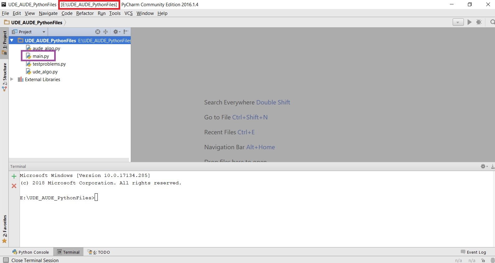
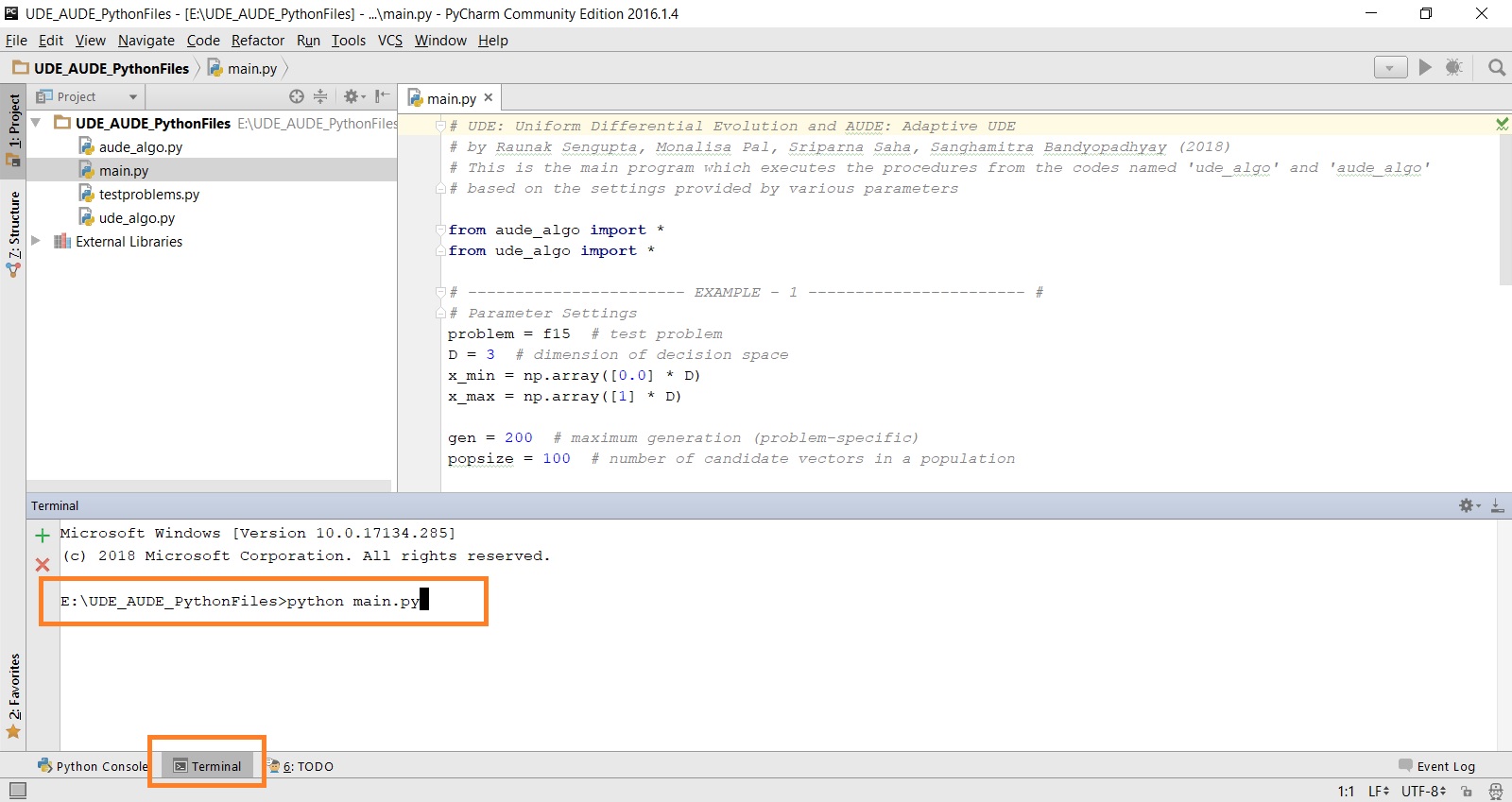
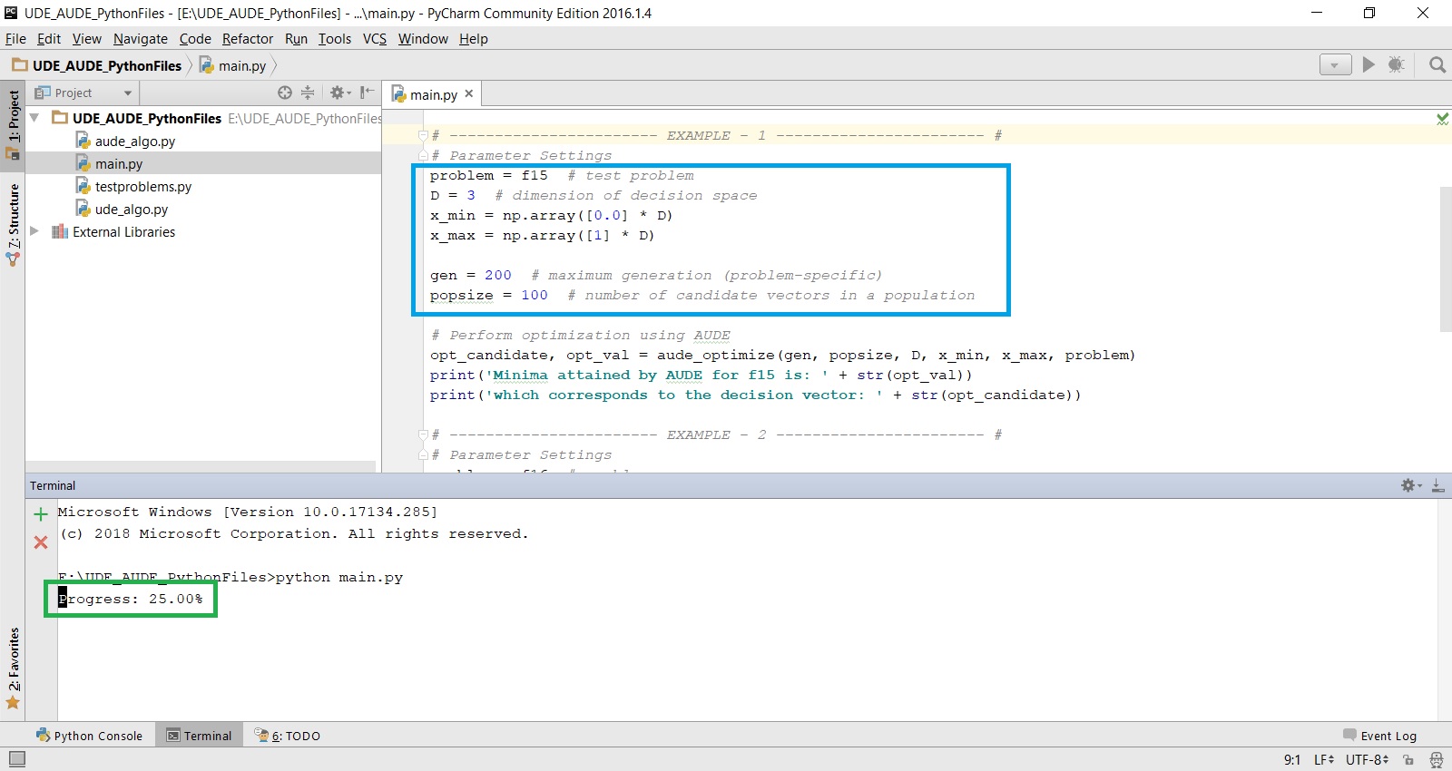
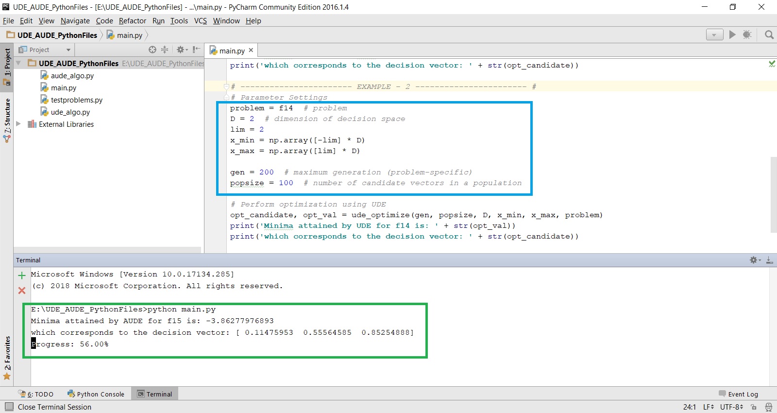
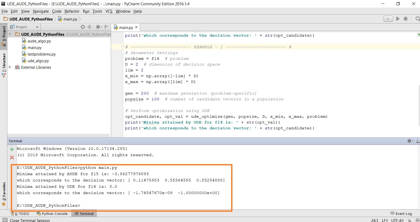
The Python 3.4 codes are available in a compressed folder named "UDE_AUDE_PythonFiles.zip" which is downloadable from the link below. The compressed folder is to be extracted in which there are 4 .py files. Out of these .py files, the file named "main.py" is to be executed and the remaining ones include function definitions required for the entire execution. The files named "aude_algo.py" and "ude_algo.py" can be used independently of each other. This program encodes test problems in "testproblems.py" file which is to be modified if some other test problems or functions of a practical applications are to be used. By default, "aude_algo.py" and "ude_algo.py" uses problems from "testproblems.py".
Click here to download the Python 3.4 implementation of AUDE and UDE.This implementation was performed on a system having Intel Core i7 processor @ 2.3GHz with 8GB RAM and using Python 3.4.
The Python 3.4 codes are available in a compressed folder named "LSHADE_cnEpSin_PythonFiles.zip" which is downloadable from the link below. The compressed folder is to be extracted in which there are 4 .py files, similar to the file structure of the proposed work. Out of these .py files, the file named "main.py" is to be executed and the remaining ones include function definitions required for the entire execution.
Click here to download the Python 3.4 implementation LSHADE‐cnEpSin.The code can be executed as listed below. Against each step, a screenshot is provided for reference. The screenshots are taken during execution of the code in Windows 10.

Visitor Counter
![]()
![]()
![]()
![]()
![]()
Author: Monalisa Pal
Email: monalisap90@gmail.com