1 / 8
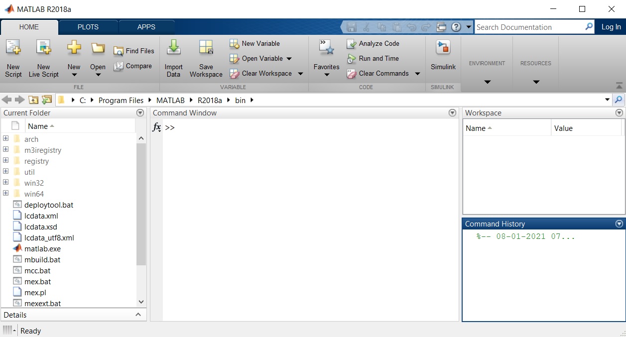
Step 1 of 8
2 / 8
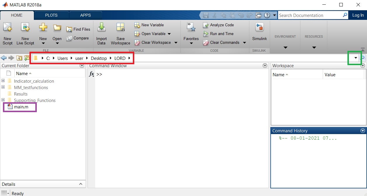
Step 2 of 8
3 / 8
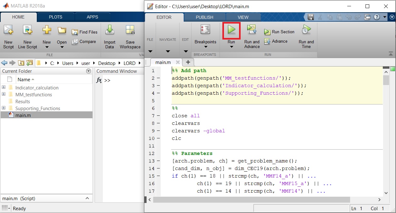
Step 3 of 8
4 / 8
Step 4 of 8
5 / 8
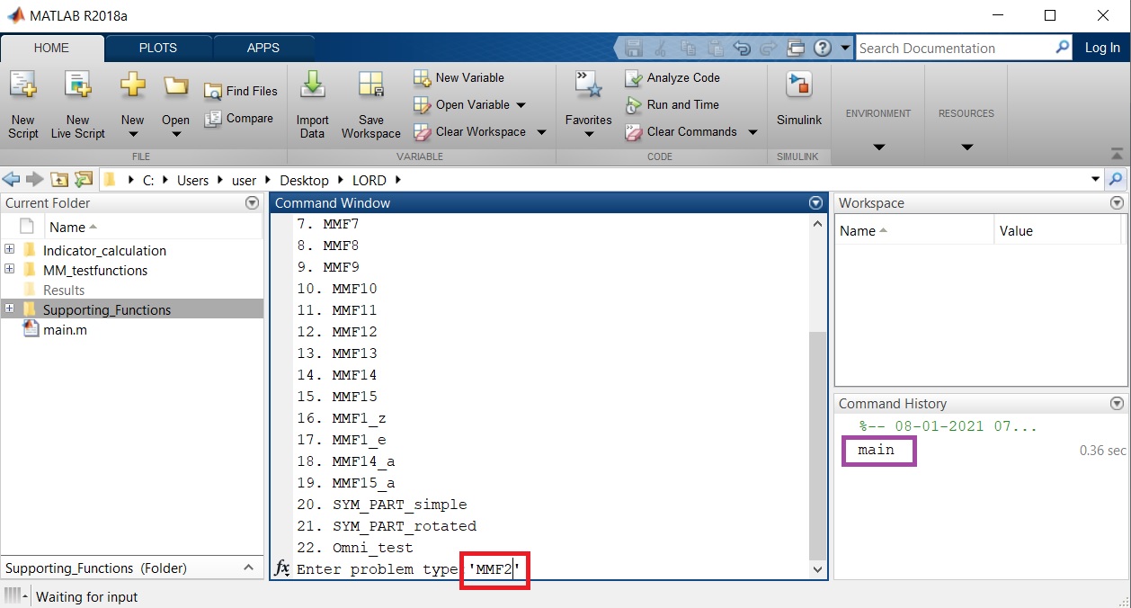
Step 5 of 8
6 / 8
Step 6 of 8
7 / 8
Step 7 of 8
8 / 8
Step 8 of 8
Welcome to this webpage which presents a multi-modal multi-objective optimization approach viz. LORD or graph Laplacian based Optimization using Reference vector assisted Decomposition. Its uses decomposition in both objective (reference vector based subspace creation) and decision (subspace clustering) space to address the many-to-one mappings from decision to objective space. The efficacy of this proposed algorithm has been analyzed on CEC 2019 competition test problems and polygon problems. The proposed work studies the scalability of LORD by varying number of objectives (upto 10), number of decision variables (upto 100) and number of solution subsets (upto 27) which can independently generate the entire Pareto-front. This webpage contains a supplementary material for describing the performance indicators used in the main manuscript, visualizing the estimated solutions, analyzing the diversity attainment behavior and comparing the outcomes with k-means clustering approach (in place of spectral clustering). This webpage also contains the MATLAB code as a downloadable ZIP folder, and the step-wise illustration for the execution of the code.
Some additional analysis and description are available for downloading as the supplementary material in the file named "Supplementary.pdf". Specifically, the supplementary material provides the following information:
Click here to download the supplementary material.
The code for LORD and LORD-II have been verified to run on MATLAB R2018a and a system having Intel Core i7 processor @ 2.2GHz and 8GB RAM.
The MATLAB codes are available in a compressed folder named "LORD.zip" which is downloadable from the link below. The compressed folder is to be extracted in which there are four folders and "main.m" file. The four folders are as follows:
Click here to download the MATLAB codes.
As LORD and LORD-II are decomposition-based approaches, the implementations are available with standard settings of sub-space partitioning. For any arbitrary sub-space partitioning, please visit this page.
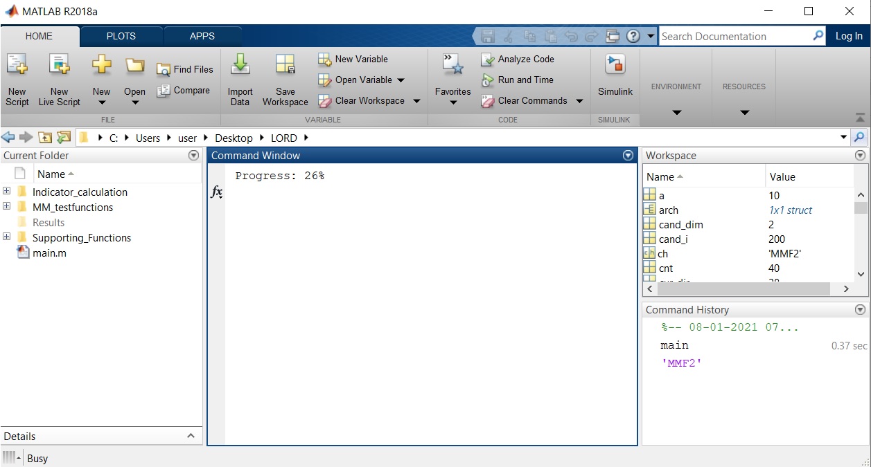
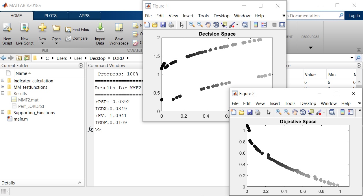
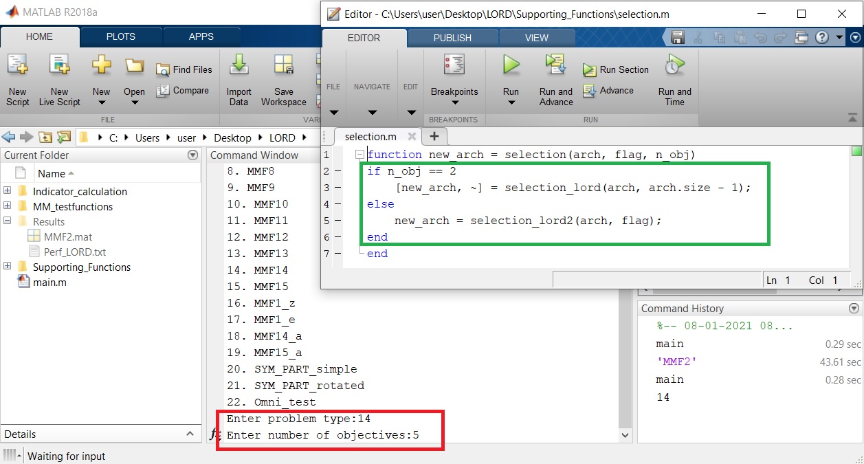
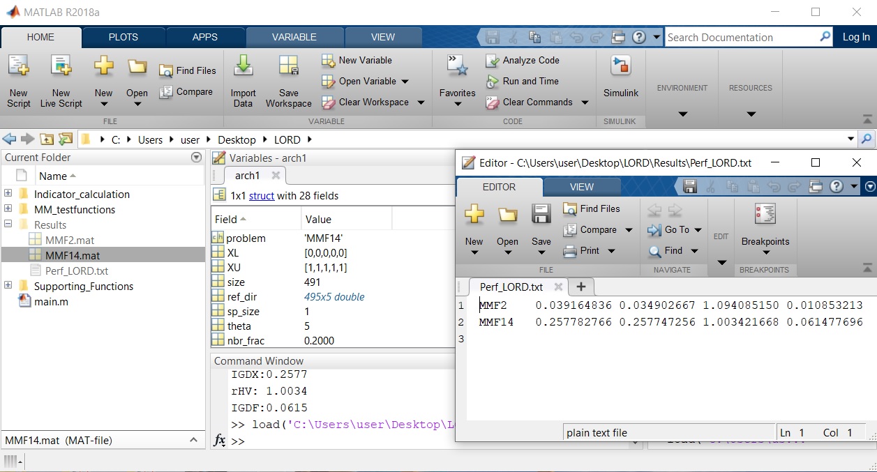
The code can be executed as listed below. Against each step, a screenshot is provided for reference. The screenshots are taken during execution of the code in Windows 10.
Visitor Counter
![]()
![]()
![]()
![]()
![]()
Author: Monalisa Pal
Email: monalisap90@gmail.com